This page serves as an entry point to everything related to Spherical Harmonics.
Contents
What are Spherical Harmonics (SH)?
According to wikipedia, SH are special functions defined on the surface of a sphere.
In computer graphics, we're using them as a tool to quickly and easily encode or decode a directional information. We use a specific set of spherical harmonics, denoted <math>Y^m_l(\theta,\phi)</math> called Laplace's spherical harmonics.
SH have interesting properties regarding their orthogonality, parity, symmetry and rotation that I will not cover here (cf. the wikipedia page for more info) as this page only is an overview. An excellent source of information is Spherical Harmonics Lighting: the Gritty Details by Robin Green that actually covers the practical use of SH for Computer Graphics, it's a well-explained extension of the original work done by Peter Pike Sloane who is pretty much the guy who introduced SH to Computer Graphics for Pre-computed Radiance Transfer (PRT).
I will rather quickly talk about how to construct the SH coefficients and how to encode/decode/convolve signals using SH.
Generalities about SH orders
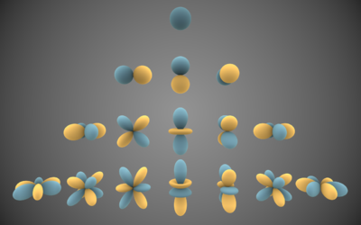
As can be seen in the inset on the right, Spherical Harmonics are functions defined over the sphere. They are denoted <math>Y^m_l(\theta,\phi)</math> where <math>l</math> is the order of the coefficient. Since SH define harmonic series, there are an infinite amount of possible orders.
For a given order <math>l</math> you have <math>2l+1</math> coefficients selected by the superscript <math>m\in[-l,+l]</math>. It ensues that the indices and amount of coefficients for each order is then:
          0           Order 0 - Total = 1 = 1²
       1  2  3        Order 1 - Total = 1 + 3 = 4 = 2²
    4  5  6  7 8      Order 2 - Total = 1 + 3 + 5 = 9 = 3²
 9 10 11 12 13 14 15  Order 3 - Total = 1 + 3 + 5 + 9 = 16 = 4²
<math>\dots</math>
We quickly see the amount of coefficients to properly represent each order grows quadratically.
Intuitively, we also can notice that the more coefficients we have, the more "directionalities" we can cover. Order 0 is a constant so it represents the "ambient term", the average response of a signal and has no specific direction. Coefficients for order 1 represent the response to a signal aligned with the X, Y and Z axes. At order 2, we start covering some diagonal directions and higher frequencies.
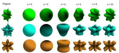
In fact, if we used an infinite sum of SH coefficients, we could encode or decode a signal perfectly. A great advantage of using SH is that we can recover a partial signal (i.e. a band-limited signal) and we will obtain a low-frequency representation of that signal, as opposed to wavelets that attempt to reconstruct all frequencies of a signal and can show high-frequency noise, a partial SH-encoded signal will always be smooth.
It is common in real-time computer graphics to use only order 2 (9 coefficients) or order 3 (16 coefficients) at most, each coefficient being a RGB float3 triplet. SH are often used to encode irradiance, which is generally spatially varying pretty smoothly. Although it varies at higher frequency than irradiance, it is also possible to encode the radiance into SH.
Actually, both radiance and irradiance are related in terms of SH, as explained by this great paper from Ramamoorthi and Hanrahan from 2001.
It was shortly followed by another seminal paper called "An Efficient Representation for Irradiance Environment Maps" that extends on the first paper and shows that order 2 SH (9 coefficients) is often enough to properly represent the irradiance field surrounding an object since additional order disappear very quickly. We will come back to these papers later as I will show an extension on this irradiance estimate to introduce the Ambient Occlusion term.
NOTE: It is sometimes desirable to express a SH coefficient <math>Y^m_l(\theta,\phi)</math> by a single index <math>Y_i(\theta,\phi)</math> where <math>i=l(l+1)+m</math>. It can be noted that <math>l(l+1)</math> gives us the "central index" (If you refer to the pyramid of coefficient indices above, these are the bold indices 0, 2, 6, 12, 20, 30, etc.) for any given order <math>l</math>, then adding <math>m</math> will address the "left" or "right" coefficients.
Inversely, when we want to retrieve <math>l, m</math> from <math>i</math> then <math>l=\lfloor\sqrt{i}\rfloor</math> and <math>m=i - l(l+1)</math>.
Constructing the SH Coefficients
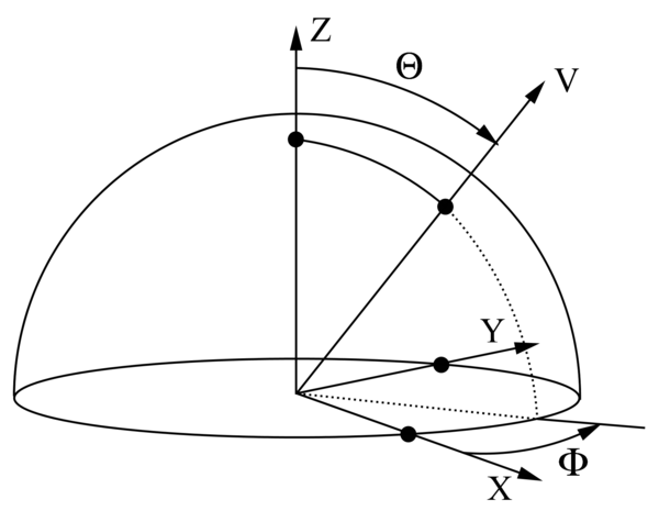
We're working with a Z-Up orientation:
The expression of vector <math>v</math> in cartesian coordinates is <math>v(\phi,\theta) = (sin(\theta)cos(\phi), sin(\theta)sin(\phi), cos(\theta))</math>.
The general spherical harmonics coefficients <math>Y^m_l(\theta,\phi)</math> are expressed as:
- <math>Y^m_l(\theta,\phi) = K^m_l P^m_l(cos(\theta)) e^{im\phi}</math>
Where <math>K^m_l = \sqrt{ \frac{(2l+1)}{4\pi}\frac{(l-m)!}{(l+m)!}}</math> is a normalization factor and <math>P^m_l(\theta,\phi)</math> is the associated Legendre polynomial.
We're interested in the real form of spherical harmonics that is given by:
- <math>Y^m_l(\theta,\phi) =
\begin{cases}
  \sqrt{2} K^{-m}_l P^{-m}_l(cos(\theta)) sin(-m\phi) & \quad \text{if } m < 0\\
   K^0_l P^0_l(cos(\theta))  & \quad \text{if } m = 0\\
  \sqrt{2} K^m_l P^{| m |}_l(cos(\theta)) cos(m\phi) & \quad \text{if } m > 0\\
\end{cases} </math>
Analytical Expressions for the first SH Coefficients
As indicated in the beginning of this page, most real-time applications only use a limited amount of SH orders (2, 3 or more rarely 4 orders) so we're usually dealing with at most 9 or 16 SH coefficients.
These coefficients have analytical expressions that we are now listing below (we dropped the <math>\theta,\phi</math> for conciseness:
- <math>
\begin{cases} \text{order }l=0\\
Y^0_0 = \frac{1}{2}\sqrt{\frac{1}{\pi}}\\
\text{order }l=1\\
  Y^{-1}_1 = \frac{1}{2}\sqrt{\frac{3}{\pi}}y & \quad m = -1\\
  Y^{0}_1 = \frac{1}{2}\sqrt{\frac{3}{\pi}}z & \quad m = 0\\
  Y^{1}_1 = \frac{1}{2}\sqrt{\frac{3}{\pi}}x & \quad m = 1\\
\text{order }l=2\\
  Y^{-2}_2 = \frac{1}{2}\sqrt{\frac{15}{\pi}}xy & \quad m = -2\\
  Y^{-1}_2 = \frac{1}{2}\sqrt{\frac{15}{\pi}}yz & \quad m = -1\\
  Y^{0}_2 = \frac{1}{4}\sqrt{\frac{5}{\pi}}(3z^2-1) & \quad m = 0\\
  Y^{1}_2 = \frac{1}{2}\sqrt{\frac{15}{\pi}}xz & \quad m = 1\\
  Y^{2}_2 = \frac{1}{4}\sqrt{\frac{15}{\pi}}(x^2-y^2) & \quad m = 2\\
\end{cases} </math>
Common Usages for SH
Signal Encoding
A signal <math>f(\theta,\phi)</math> whose value is available for all directions can be encoded (or rather, projected) into SH coefficients by estimating the following integral:
- <math>C_i = \int_0^{2\pi}{\int_0^{\pi} {f(\theta,\phi)Y_i(\theta,\phi)sin(\theta)} \mathrm{d}\theta \mathrm{d}\phi}</math>
To implement this integration numerically we can use the naïve pseudo-code:
float EncodeSHCoeff( int l, int m ) {
	const int STEPS_PHI = 200;
	const int STEPS_THETA = 100;
	const float dPhi = 2*PI/STEPS_PHI;
	const float dTheta = PI/STEPS_THETA;
	float coeff = 0.0f;
	for ( int i=0; i < STEPS_PHI; i++ ) {
		float phi = i * dPhi;
		for ( int j=0; j < STEPS_THETA; j++ ) {
			float theta = (0.5f+j) * dTheta;
			float value = EstimateFunction( phi, theta );
			float SHvalue = EstimateSH( l, m, phi, theta )
			coeff += value * SHValue * sin( theta ) * dPhi * dTheta;
		}
	}
	return coeff;
}
A better (and faster!) way to do that would be to use importance sampled Monte Carlo sampling. Please refer to Robin Green's paper for details about the technique.
We first need to generate an arbitrary set of samples on the sphere. We choose the samples so that they are uniformly distributed on the sphere, thus ensuring that each sample carries the same weight that will be <math>\frac{4PI}{N} \text{ where } N \text{ is the amount of samples}</math>:
struct sample_t {
	float3	direction;
	float	theta, phi;
	float*	Ylm;
};

void PreComputeSamples( int sqrt_n_samples, int n_bands, sample_t samples[], float ) {
	// fill an N*N*2 array with uniformly distributed samples across the sphere using jittered stratification
	int i = 0; // array index
	double oneoverN = 1.0 / sqrt_n_samples;
	for ( int a=0; a < sqrt_n_samples; a++ ) {
		for ( int b=0; b < sqrt_n_samples; b++ ) {
			// Generate unbiased distribution of spherical coords
			double x = (a + random()) * oneoverN; 			// Do not reuse results
			double y = (b + random()) * oneoverN; 			// Each sample must be random!
			double theta = 2.0 * acos( sqrt( 1.0 - x ) );	// Uniform sampling on theta
			double phi = 2.0 * PI * y;						// Uniform sampling on phi

			// Convert spherical coords to unit vector
			samples[i].direction = float3( sin(theta)*cos(phi), sin(theta)*sin(phi), cos(theta) );
			samples[i].theta = theta;
			samples[i].phi = phi;

			// precompute all SH coefficients for this sample
			for ( int l=0; l < n_bands; ++l ) {
				for ( int m=-l; m<=l; ++m ) {
					int index = l*(l+1)+m;
					samples[i].Ylm[index] = EstimateSH( l, m, theta, phi );
				}
			}
			++i;
		}
	}
}
Signal Decoding
@TODO:
Signal Convolution
@TODO:
Signal Triple Product
@TODO:
Triple Product of Zonal and Spherical Harmonics
@TODO:
About Distant Radiance and Irradiance Environment
As mentioned
Archives
You can find an old (2009) explanation about SH Environment Maps.


