| Line 649: | Line 649: | ||
To sum up : | To sum up : | ||
| − | <math>Li(P,\vec\omega) = \mathbf{p^\prime}(\widehat{\vec\omega \vec\omega_{sun}}) e^{-\tau(\vec\omega_{sun})} L_{sun}(\vec\omega_{sun})</math> | + | <math>Li(P,\vec\omega) = \mathbf{p^\prime}(\widehat{\vec\omega \vec\omega_{sun}}) e^{-\tau(P,\vec\omega_{sun})} L_{sun}(\vec\omega_{sun})</math> |
where : | where : | ||
| − | <math>\tau(\vec\omega_{sun}) = \boldsymbol{\sigma} \boldsymbol{\rho}(x)</math> | + | <math>\tau(x,\vec\omega_{sun}) = \boldsymbol{\sigma} \boldsymbol{\rho}(x)</math> |
<math>\boldsymbol{\sigma}</math> is the global cloud extinction factor | <math>\boldsymbol{\sigma}</math> is the global cloud extinction factor | ||
<math>\boldsymbol{\rho}(x)</math> is the accumulated density at <math>x</math> we talked about earlier | <math>\boldsymbol{\rho}(x)</math> is the accumulated density at <math>x</math> we talked about earlier | ||
Revision as of 14:54, 1 April 2011
This page talks about the complex task of rendering clouds in real-time. It's more of a guide through my own experience rather than an extensive review of all existing techniques. The target audience is the skillful amateurs of the demoscene and video games developers community rather than the expert scientists writing articles for the Siggraph, and I hope I didn't make too many mistakes in the various formulas and statements used herefater.
First you must know that I've been in love and studied clouds for a pretty long time now. I remember first taking pictures of sunsets from my bedroom window when I was 15, I'm now 35 and nothing has changed : I'm still amazed by the variety of colors and shapes that clouds can bring to an otherwise "sad" blue sky.
My favorites are the storm clouds : the humongous cumulo-nimbus.
- Chapter 1 and 2 are an introduction to cloud shapes and complex lighting physics occurring within them.
- Chapter 3 concentrates on some rendering algorithms I have tested.
Contents
- 1 Cloud Types
- 2 Rendering
- 3 Several Lighting Methods
Cloud Types
When it comes to rendering, you have 2 difficulties to overcome : lighting and shape. Both are difficult and very important.
You may underestimate the importance of the shape of a cloud, especially because they look random so you might think a random shape is okay. But then you are plain wrong, because clouds are all but random.
Shape
If you watch a time-lapse video of a cloud, you can see how clouds move, how they are created and destroyed. One main observation to make is that accelerated clouds motion make them look like regular smoke. This is an important fractal pattern : clouds are like smoke, but bigger. And as they are orders of magnitude larger, the time scale is orders of magnitude smaller. It will take several minutes for the huge mass of a cloud to accomplish the same motion as smoke. A bit like the time for humans seems like slow motion when compared to insects.
You can see in the example video above how the cloud is "pulsed" from hot air pockets below. You can also see how there are "sources" and "sinks" that make the cloud appear and disappear.
All these obey the complex laws of thermodynamics : hot humid air rises up and evaporates while cold air falls down and liquefies, all these occurring at precise temperature and pressure, depending on the altitude.
Clouds are composed mainly of water in all its states : gas (i.e. water vapor), liquid (i.e. small droplets) and solid (i.e. snow and ice crystals). Clouds also need "nuclei" particles to form, like dust or aerosol molecules : despite large humidity quantities in the air, if there is no nuclei (i.e. the air is too clean), there won't be any cloud.
Every Altitude its Cloud
Most of the clouds are very compact and fit in a "tiny" altitude range, although the storm cumulo-nimbi clouds span the entire range of altitudes, some of them going up to 15 kilometers (!!).
The scales in these clouds vary dramatically. Thin clouds are easily traversed by light while thick clouds are mostly reflective. Light scattering in clouds is really important because of the scales browsed by clouds : a photon doesn't go in a straight line for a long time when pacing through the many hundreds of meters inside a cloud.
Several ways for modeling clouds
Please, read the excellent Ken Perlin's presentation so you get familiar with the different Perlin noises.
Some are great for introducing regular randomness (plain noise), some others are good for clouds (sum 1/f(noise)) while even others are good for terrain modeling (sum 1/f(|noise|)) and are given funny names like "ridged multi fractal" or "fractal brownian motion".
Once you have your basic noise function, it's all a matter of intelligently combining several noises at different amplitudes and frequencies.
Alto/Cirro cumulus & stratus
These are thin vaporous high-altitude clouds. They are the easiest and most commonly simulated clouds because they are very thin and can be easily mapped to a plane, as shown on the image below.
For alto/cirro cumulus forms, there is a clear distinct "cauliflower" pattern that Perlin noise can easily achieve using the Turbulence pattern, as shown below :
For a great introduction to the complex light scattering within clouds, and the rendering of thin cloud slabs, I invite you to read the (quite technical) paper "Real-time realistic illumination and shading of stratiform clouds" by Bouthors et al.
You're okay sticking to a 2D cloud plane (even faking thickness through parallax mapping), you can even simulate up to the already thick stratocumulus until you need to display distinct clumps, holes or fly through the clouds. From this point on, you need to really render 3D clouds.
Nimbostratus, Cumulus & Cumulo-nimbus
These are the big guys (and my favorite ![]() ) !
) !
I remember being baffled by the foundation paper "A Simple, Efficient Method for Realistic Animation of Clouds" by Dobashi et al. in 2000, where these guys managed to render impressively realistic clouds using particles, while the clouds were modeled using a cellular automaton. This paper served as a base for Mark Harris and his well known clouds.
This team of Japanese, when it comes to imitating reality, is really excellent ! They are also responsible for the foundation paper "Display of The Earth Taking into Account Atmospheric Scattering" about the sky model later implemented in real time by Sean O'Neil. On the downside though, like me, their english sucks and I remember re-reading 10 times the same sentence to try and understand what they meant.
Best way yet : CFD
Computational Fluid Dynamics, in my opinion, is yet the best way to achieve great cloud simulation. I never actually tried large scale 3D CFD simulations but the few ones I've experimented with allowed me to create a pretty convincing smoke plume. And as stated earlier, clouds are nothing more than smoke in slow-motion. All you have to do is to create a sufficiently large 3D playground, model wind, hot air rising, cool air falling down and advect water droplets and various parameters along the resulting velocity fields. I'm pretty sure this will create really great clouds !
The only problems are :
- Memory <math>\to</math> I'm not sure we're ready yet to experiment on volumes the size of a city for real-time applications
- Scalability <math>\to</math> Splitting the computation to multiple GPU threads. I bet Compute Shaders and Cuda could help on that but I don't know anything about them. A good thing though is that clouds evolve slowly, so updating a new cloud state every 30 seconds is quite okay (except for dramatic fast-forward effects that might occur in games).
Many tests through the years
Of course, I experimented with cloud particles myself at that time and I obtained some nice results but these clouds always kinda lacked the fluffiness I was after. This I learned : you can't really have great fluffy clouds with particles. First because of their disjoint nature (you're not using a mesh or tracing through a continuous volume here, merely splatting flat stuff together), then because of the lighting model that failed to account for important scattering events. Basically, with real-time particle models, you can take into account extinction and 0- or single-scattering events so you get the main features of a cloud, but you lack the general "denseness" and solid-feeling of cumuli and cumulo-nimbi clouds.
I tried many things, with more or less satisfying results :
- Soft particles with precomputed Spherical Harmonics lighting, the lighting was quite okay but the clouds were obviously too "solid looking"
- Marching cubes and other "mesh clouds" rendering, my intention was to render these in several depth buffers seen from front and back and to "subtract" the depths so I obtained the thickness of the mesh at a particular point in space (I first had this idea in 1995 and managed to have one of the first real-time volumetric light effects ever with my software renderer, I never used it in a demo though and the effect has since been re-used countless times). This could have worked but only computing the absolute thickness of an object, without accounting for holes and concavities always yielded poor results where it seemed light "poured through the volume" and although you got interesting god ray effects, the rendering was really not looking anything like a cloud.
- Mega-particles, I first encountered this "technique" about 6 months ago (like november 2010) and, although I couldn't see how the effect worked (it looked like quite a "I bullshit you" effect), I decided to give it a try. This yielded interesting results but not because of the effect itself, as it's mainly a post-process and rendering a 3D cloud as if it was a 2D plane gives nasty "scrolling artefacts" when you move the camera. No, the main interesting rendering achievement here was because it was the first time I really correctly used phase functions AND a now quite old technique called "Deep Shadow Maps". This is really an interesting read !
For clouds modeling, I wrote a "recursive sphere aggregation" software where you drew your base cloud shape using big spheres, then the software created smaller "level 1" spheres on the surface of the these "root spheres" and simulated auto-spacing, then recursively created smaller "level 2" spheres and simulated again, and so on... I managed to obtain nice cloud shapes with that software but I the rendering was awful. I never managed to have a nice rendering AND modeling at the same time...
Until finally...
It's only recently that I finally came up with the actual way of rendering nice volumetric clouds, some that you can change dynamically and view from anywhere, even from inside !
To do this, there is no other solution than rendering a 3D volume : a volume that tells you for each position in space whether or not there is a density of "cloud material". It's also very recently that it has become quite tractable to use 3D textures and even more recently that shaders allow you to perform ray-marching steps, the first examples of this being parallax mapping that is simply "terrain marching" to find the intersection of a ray with a height field.
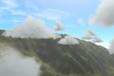
A couple years ago, my friend David (U2/Popsy Team) really was the first one to come up with super nice real-time clouds by ray-marching a volume, as seen in the picture below. His technique is a mix of mesh rendered into a volume texture, coupled with pre-computed spherical harmonics for lighting and various real-time 2D noise for shape variations, and that's brilliant !
Rendering
You don't change a winning team : ray-marching a volume texture is the key to realistic 3D clouds.
Ray-marching
The absolute key to a nice ray-marching is the amount of steps you use. The more the better !
For a nice rendering I needed about 128 steps but you can't write a shader with a for loop of 128 steps for a 1024x768 surface so I exploited another great feature of clouds : their low frequency nature. The fact that clouds are large and only display small changes in shape made me guess about the impact of rendering not a 1024x768 surface but a downscaled version of 256x192 (downscaled by a factor 4). Ray-marching 128 steps in such a small surface doesn't change the impression that you are looking at clouds, and helps you to maintain a steady and fast frame rate.
On top of that, the downscale factor gives a very flexible way to scale the time used by the effect. For low end machines you can downscale by 8, for very high end machines you can downscale by 2. It's all a matter of experimenting with various hardware and use a scale factor appropriate for both the machine and the time you want to allocate to render clouds (as for most games, you can't spend your entire time on rendering).
So the first trick is this : render low, render fast !
Review of Light Behavior
First, let's review the basics of light behavior within a participating medium. I couldn't advise you more to read the great book "Realistic Image Synthesis using Photon Mapping" by Henrik Wann Jensen, to which I refer to as soon as I hit an obstacle or forget something (which is, I confess, most of the time).
To be quick, light goes into straight lines unless it encounters an obstacle, in which case it's either absorbed or scattered in any direction. The choice in scattering direction is quite arbitrary, depends on many parameters like surface smoothness or, in the case of a participating medium (i.e. water, smoke, dust), the type and size of particles the light is traversing :
- Small air molecules won't absorb light very much unless on very long distances, like from the ground to the upper atmosphere. And it will do so differently depending on the wavelength (which is the reason why the sky is blue). The theory for light scattering by gas molecules is the Rayleigh scattering theory.
- Large aerosols like dust and microscopic water droplets will rather absorb (i.e. smoke or dust) or reflect/refract (i.e. water droplets) light and will do so on much smaller distances than air molecules. The theory for light scattering by large aerosol particles is the Mie scattering theory.
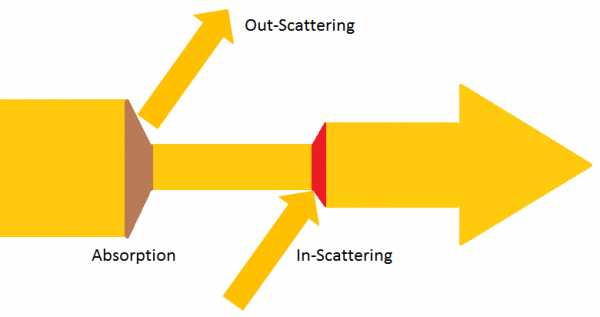
Light, by going through a participating medium will then suffer 2 things :
- Absorption. Light is absorbed and transformed into something else, like heat. The amount of absorption suffered by light over a distance is given by <math>\sigma_a</math> (sigma "a", for absorption)
- Scattering. Light is reflected in any direction. The amount of scattering suffered by light over a distance is given by <math>\sigma_s</math> (sigma "s", for scattering)
The combination of absorption and scattering is called the extinction. The amount of extinction suffered by light over a distance is given by <math>\sigma_t = \sigma_a + \sigma_s</math>, the extinction coefficient.
Extinction
Extinction is multiplicative by nature : you constantly lose energy as you advance inside the medium and light extinction is given by :
<math>L(x,\vec\omega) = e^{-\tau(x,x+\vec\omega\Delta_x)} L(x+\vec\omega\Delta_x,\vec\omega)</math>
<math>\tau(x,x^\prime) = \int_x^{x^\prime}\sigma_t(s)\, ds</math>

where :
<math>x</math> denotes the current position
<math>\vec\omega</math> denotes the view direction
<math>\Delta_x</math> represents the distance the light marched through the medium
<math>\tau(x,x^\prime)</math> is called the optical depth. If your medium has a constant density between <math>x</math> and <math>x^\prime</math>, then the optical depth is simply : <math>\tau(x,x^\prime) = \sigma_t\left | xx^\prime \right\vert</math>
<math>L(x,\vec\omega)</math> is the energy that reaches the position <math>x</math> in the direction <math>\vec\omega</math> and is called the radiance
Here, <math>L(x+\vec\omega\Delta_x,\vec\omega)</math> is the radiance that enters the back of the considered volume <math>\Delta_x</math> meters away from <math>x</math> in the view direction <math>\vec\omega</math>.
As an example, if your extinction coefficient is constant in your medium, it's equivalent to write :
<math>e^{\sigma_t\Delta_x} = e^{\sigma_t\frac{\Delta_x}{2}}\cdot e^{\sigma_t\frac{\Delta_x}{2}}</math>
That means you get the same result by performing a single large ray-marching step compared to performing 2 small ones. As a result, we see that it's not important to trace more steps than necessary if no change in the medium's properties exist.
Extinction is one of the 2 results that come out of the ray-marching process. As light's extinction will slightly vary with wavelength, it's visually important to store the extinction factor as a RGB vector. But it's still quite acceptable to store extinction as a single luminance factor as we will see below when we will combine extinction and in-scattering.
In-Scattering
In-scattering is the amount of light that gets 'added' to the existing light along the way. Of course we lose some energy because we hit some particles, but we also gain some other that bounced off of nearby particles. That's all a game of statistics really. ![]()
The expression for in-scattering is much more complicated than extinction and is the main reason why lighting is a difficult process :
<math>L(x,\vec\omega) += \int_{x}^{x+\Delta_x\vec\omega}e^{-\tau(x,x^\prime)}\sigma_s(x^\prime)\int_\Omega p(x^\prime,\vec\omega,\vec\omega^\prime)L(x^\prime,\vec\omega^\prime) \, d\vec\omega^\prime \, dx^\prime</math>
Wow that's a big one ! (but at least, notice the not very mathy "+=" operator meaning this part is added to the previously seen radiance, attenuated by extinction)
To make things simpler, we can rewrite it this way :
<math>L(x,\vec\omega) += \int_{x}^{x+\Delta_x\vec\omega}e^{-\tau(x,x^\prime)}\sigma_s(x^\prime) L_i(x^\prime,\vec\omega) \, dx^\prime</math>
Basically, this means that along a path, light gets decreased by extinction (the <math>e^{-\tau(x,x^\prime)}</math> part) but also gets added from other directions (the <math>L_i(x^\prime,\vec\omega)</math> part).
<math>L_i(x^\prime,\vec\omega)</math> is what I call the incoming irradiance which is the contribution of radiances from all directions about <math>x^\prime</math> that get somehow reflected in the view direction <math>\vec\omega</math>, the probability of such reflection is given by the phase function that we will describe later.
This is the infamous radiosity that was for a long time approximated by a single ambient term, by lack of methods or computing power to solve this complicated equation.
So, to sum up, light along a very short step <math>\Delta_x</math> where the medium properties are constant gets added with some in-scattered radiance :
<math>L(x,\vec\omega) += e^{-\sigma_t\Delta_x} \sigma_s(x) \Delta_x L_i(x,\vec\omega)</math>
The same way extinction was multiplicative by nature, in-scattering is additive by nature.
In-Scattering is the second one of the 2 results that come out of the ray-marching process. Although extinction is only slightly affected by wavelength and could well be stored as a single factor, in-scattering on the other hand strictly needs to be stored as a RGB vector (that is, if you want your sky to be blue by day and orange at sunset) (who knows ? That might come handy).
Combining Extinction & In-Scattering
Again, for a very short step <math>\Delta_x</math> where the medium properties are constant, we can finally write the radiance :
<math>L(x,\vec\omega) = \sigma_s(x) \Delta_x L_i(x,\vec\omega) + e^{-\sigma_t\Delta_x} L(x+\Delta_x\vec\omega,\vec\omega)</math>
We see that it all comes down to :
- Perform extinction of the radiance at the start of the marching step (i.e. <math>e^{-\sigma_t\Delta_x} L(x+\Delta_x\vec\omega,\vec\omega)</math>)
- Add in-scattered radiance along the marching step (i.e. <math>\sigma_s(x) \Delta_x I(x)</math>)
You can view the light ray-marching process as gaining some energy (i.e. in-scattering, an addition) then marching a little and losing some energy (i.e. extinction, a multiplication).
We can rewrite the equation above in terms of discrete ray-marching steps :
<math>L(i) = \sigma_s(i) \Delta_x L_i(i) + e^{-\sigma_t(i)\Delta_x} L(i-1)</math>

Where :
<math>i</math> is the index of the ray-marching step.
<math>L(0)</math> is the background radiance we start with. It's basically the color of your pre-rendered scene.
Let's write a few steps of ray-marching using the above notation :
Step 0:
 <math>L(0) = BackgroundRadiance</math>

Step 1:
 <math>L(1) = \sigma_s(1) \Delta_x L_i(1) + e^{-\sigma_t(1)\Delta_x} L(0)</math>

Step 2:
 <math>\begin{align}L(2)
& = \sigma_s(2) \Delta_x L_i(2) + e^{-\sigma_t(2)\Delta_x} L(1) \\
& = \sigma_s(2) \Delta_x L_i(2) + e^{-\sigma_t(2)\Delta_x} \big[ \sigma_s(1) \Delta_x L_i(1) + e^{-\sigma_t(1)\Delta_x} L(0) \big] \\
& = \sigma_s(2) \Delta_x L_i(2) + e^{-\sigma_t(2)\Delta_x} \sigma_s(1) \Delta_x L_i(1) + e^{-\sigma_t(2)\Delta_x} e^{-\sigma_t(1)\Delta_x} L(0) \\
\end{align}
</math>
Step 3:
 <math>\begin{align}L(3)
& = \sigma_s(3) \Delta_x L_i(3) + e^{-\sigma_t(3)\Delta_x} L(2) \\
& = \sigma_s(3) \Delta_x L_i(3) + e^{-\sigma_t(3)\Delta_x} \big[ \sigma_s(2) \Delta_x L_i(2) + e^{-\sigma_t(2)\Delta_x} \big[ \sigma_s(1) \Delta_x L_i(1) + e^{-\sigma_t(1)\Delta_x} L(0) \big] \big] \\
& = \sigma_s(3) \Delta_x L_i(3) + e^{-\sigma_t(3)\Delta_x} \sigma_s(2) \Delta_x L_i(2) + e^{-\sigma_t(3)\Delta_x} e^{-\sigma_t(2)\Delta_x} \sigma_s(1) \Delta_x L_i(1) + e^{-\sigma_t(3)\Delta_x} e^{-\sigma_t(2)\Delta_x} e^{-\sigma_t(1)\Delta_x} L(0) \\
\end{align} </math>
and so on...
Each step brings us forward toward the camera, where we obtain the final radiance reaching the sensor.
From the recurrence relation above we see that, if we perform N steps of ray-marching :
<math>Extinction(N) = \prod_{i=1}^N e^{-\sigma_t(i)\Delta_x}</math>
<math>InScattering(N) = \sum_{i=1}^N \mathbf{K}(i) \sigma_s(i) \Delta_x L_i(i)</math>

where :
<math>Extinction(0) = 1</math>
<math>InScattering(0) = BackgroundRadiance</math>
<math>\mathbf{K}(i) =
\begin{cases}
{\prod_{j=i+1}^N e^{-\sigma_t(j)\Delta_x}} & i < N \\
1 & i = N
\end{cases}
</math>
And finally, after N steps :
<math>\begin{align}L(\vec\omega) & = InScattering(N) + Extinction(N) * InScattering(0) \\
& = InScattering(N) + Extinction(N) * BackgroundRadiance \\
\end{align}</math>

where :
<math>BackgroundRadiance</math> is the color of your pre-rendered scene
What I usually do is to cumulate the extinction and in-scattering as 2 distinct RGB values. The pseudo-code for ray-marching goes something like this :
void  RayMarch( float3 _In, float3 _View, float _Distance, float3& _Extinction, float3& _InScattering )
{
  float3  Step = _View * _Distance / (N+1);       // Our march step
  float   StepSize = length(Step);                // Size of a unit step
  float3  CurrentPosition = _In + (N+0.5) * Step; // Start at the end of the ray

  _Extinction = 1.0;   // We start with full energy as we have not entered the medium yet...
  _InScattering = 0.0; // ...but no in-scattered energy yet
  for ( int StepIndex=0; StepIndex < N; StepIndex++ )
  {
    // Get extinction & scattering coefficients at current position
    float3 Sigma_t = GetExtinctionCoeff( CurrentPosition );
    float3 Sigma_s = GetScatteringCoeff( CurrentPosition );

    // Compute extinction for our single step
    float3 CurrentStepExtinction = exp( -Sigma_t * StepSize );

    // Perform extinction
    _Extinction *= CurrentStepExtinction;  // Current extinction is multiplied with existing, cumulative extinction

    // Perform in-scattering
    _InScattering += CurrentStepExtinction * Sigma_s * StepSize * ComputeRadiance( CurrentPosition, _View ); // In-scattering is accumulated to existing in-scattered energy

    // March one step backward
    CurrentPosition -= Step;
  }
}
Note that we ray-march backward, starting from the rear and ending at the camera. By slightly rewriting the code it's easy to march forward but I find the backward method more intuitive (no, I'm not gay ! Be serious for a minute there, it's important stuff).
As I said earlier : it's quite okay to discard the RGB nature of extinction and store it as a single luminance factor. If you do so, you end up with a RGB vector of in-scattered energy and a single value for extinction that you can store in Alpha.
You can then combine the resulting RGBA image with any existing buffer (i.e. your pre-rendered scene) using the pre-multiplied alpha blend mode :
TargetColor = TargetColor * SourceAlpha + SourceColor
Which has the same effect as writing :
NewColor = BackColor * Extinction + InScattering
NOTE : Notice that in-scattering has already been multiplied by extinction during ray-marching so it would be plain wrong to multiply it again afterward by (1-Extinction) so this is not the same as using the standard alpha blend mode !
The missing functions
In the pseudo-code above, I used 3 mysterious functions :
- GetExtinctionCoeff()
- GetScatteringCoeff()
- ComputeRradiance()
Well, if you can read, they're not that mysterious... The first 2 retrieve the extinction/scattering coefficients at a given position. If you modeled your clouds from a density function <math>\rho(x,y,z)</math> then :
<math>\sigma_t = \rho(x,y,z) \boldsymbol{\sigma}</math>
<math>\sigma_s = \rho(x,y,z) \kappa \boldsymbol{\sigma}</math>

where :
<math>\boldsymbol{\sigma}</math> is the global extinction factor that gets modulated by density
<math>\kappa</math> is the scattering to extinction ratio or albedo, that should always be < 1 to be physically accurate (in the case of clouds, we saw that it was nearly 1)
In my case, the density <math>\rho(x,y,z)</math> is obtained from Perlin noise stored in a 3D texture :
float GetDensity( float3 _Position )
{
  float RawDensity = 0.0;
  float Amplitude = 1.0;
  for ( int OctaveIndex=0; OctaveIndex < OCTAVES_COUNT; OctaveIndex++ )
  {
    RawDensity += Amplitude * Perlin( _Position );  // Fetch Perlin noise value from 3D texture
    Amplitude *= 0.5;  // Halve the amplitude
    _Position *= 2.0;  // Double the frequency
  }

  return saturate( RawDensity - DensityOffset );
}
I usually use a 16x16x16 Perlin noise texture, which I combine with a function like GetDensity() above. Anyway, to avoid OCTAVES_COUNT texture taps, I pre-computed a 128x128x128 texture that encodes 4 octaves and allows me to retrieve the density in a single tap at the cost of increased memory usage.
The really tricky part is the ComputeRadiance() function. This is where the real cloud lighting takes place.
Scattering Within a Cloud
If you remember the daunting integral for in-scattering, you may recall that we simplified it by reducing the inner integral to :
<math>L_i(x,\vec\omega) = \int_\Omega p(x,\vec\omega,\vec\omega^\prime)L(x,\vec\omega^\prime) \, d\vec\omega^\prime</math>

where :
<math>x</math> is the current position for computing incoming radiance
<math>\Omega</math> is the entire sphere of incoming directions
<math>\vec\omega</math> is our view direction, the outgoing direction in which we view radiance
<math>\vec\omega^\prime</math> is a specific incoming direction
This integral is "simply" a matter of computing how the incoming radiance arriving in direction <math>\vec\omega^\prime</math> is redistributed in outgoing (i.e. view) direction <math>\vec\omega</math>.
The function <math>p(x,\vec\omega,\vec\omega^\prime) = p(x,\theta)</math> with <math>\theta = \widehat{\vec\omega \vec\omega^\prime}</math> the angle between the incoming and outgoing direction, is called the phase function.
For a cloud, it looks something like this :
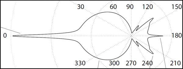
This is what I call the Watoo-Watoo phase function (from, an old cartoon I used to watch when I was a kid).
NOTE: This phase function has been created using the excellent MiePlot software by Philip Laven (http://www.philiplaven.com/mieplot.htm)
We can observe from this phase function that :
- There is a strong forward peak that concentrates 50% of the incoming energy, so the path of light in a cloud is barely altered
- There is a wide forward peak (48% of the scattering) that creates a fairly isotropic scattering in the forward direction
- There is a sudden medium peak at about 140° (backward) that is responsible for the fogbow
- There is a narrow backward peak at about 179° that is responsible for the glory
The phase function has the interesting property that <math>\int_\Omega p(x,\vec\omega,\vec\omega^\prime) \, d\vec\omega^\prime = 1</math>, ensuring all energy arriving at a point is scattered in all directions without loss or gain : conservation.
Anyway, the important point here is that to evaluate <math>L_i(x,\vec\omega)</math> you need to know <math>L(x,\vec\omega^\prime)</math> in all directions <math>\vec\omega^\prime</math> arriving at <math>x</math>. And we saw earlier that to compute radiance <math>L(x,\vec\omega^\prime)</math>, you need to integrate (i.e. ray-march) through the cloud...
It means that damn inner-integral introduces recursivity ! For each ray-marching step, you must cast M other rays around and ray-march them again, and for each these secondary ray-marchings, you need to cast M rays around and ray-march them too, and so on !
If you integrate <math>L(x,\vec\omega^\prime)</math> only once, that means you account for single-scattering events : light that has bounced only once, then exited the cloud.
If you ray-march along the <math>\vec\omega^\prime</math> direction and at each step you integrate <math>L(x,\vec{\omega^{\prime\prime}})</math> (recursion level 1), that means you account for single and double-scattering events : light that has bounced either once or twice, then exited the cloud.
I let you guess the next one... But YES ! That's hell ! Here is the algorithm for such a nightmare :
function RayMarchingHell( float3 _In, float3 _View, float _Distance ) : SomeResultYou'llNeverGetAnyway
{
  float3 Position = _In;
  float3 Step = _View * _Distance / N;
  float  ImprobableResult = 0.0;
  for ( int StepIndex=0; StepIndex < N; StepIndex++ )
  {
    for ( int DirectionIndex=0; DirectionIndex < M; DirectionIndex++ )
    {
       float3 Direction = PrecomputedDirection[DirectionIndex];                    // Some direction on the sphere of directions
       float  Distance2Exit = ComputeExitDistance( Position, Direction );          // Distance 'til we exit the cloud
       ImprobableResult += RayMarchingHell( Position, Direction, Distance2Exit );  // Infernal recursion !
    }

    Position += Step;  // March (but you'll never get there anyway)
  }

  return ImprobableResult;
}
Who said quantum computing ?
0- and Single-Scattering Events
By observing the Watoo phase function, we can notice that there is a strong forward peak (i.e. the Watoo's beak) which, according to Bouthors et al. account for half the intensity.
This means light is, for a large part, statistically unaffected by going through the cloud. This forward peak is responsible for the silver lining visible the the edges of certain clouds because the thickness at edges is small and only few scattering events occur.
HINT: If you decide to somehow use a low frequency encoding for cloud radiance, like Spherical Harmonics or SRBF for example, it's ill advised to include the strong forward peak in the encoding. Indeed, it's far better to encode 50% of the energy, scattered by the Watoo phase function with its beak cut off (i.e. general, "isotropic" scattering). Then you can add the remaining 50% strong-forward energy through standard directional lighting and (extinction + 0- and single-scattering) through the cloud.
A 0-scattering event is simply the light going through the cloud without encountering any matter (i.e. transparency), while single-scattering events are the light being reflected exactly once in the view direction before exiting the cloud and are easy to compute analytically (cf. again the excellent paper by Bouthors et al.).
Further Scattering Events
Although you can find additional smart ways to compute higher order scattering events in the paper by Bouthors et al., they are mainly limited to their stratiform clouds model.
The truth is revealed in the sequel to the stratiform clouds paper : Interactive multiple anisotropic scattering in clouds.
These clouds kick some serious ass !... But you get a cold shower once you have read the paper. Indeed, the simulation required a few weeks of computation and yielded a 25Gb database that the team later decimated into an horrible formula necessitating 7 different textures (as far as I remember).
So okay, plenty of data, that were later processed to find interesting correlations which finally led to breaking down the original 25Gb to a more tractable solution. But yielding a formula that has nothing to do with a classical lighting equation anymore... That's more of a technical prowess rather than an algorithmic leap.
Anyway, the paper is really interesting to read and offers nice solutions for finding the most probable path of photons given a piece of volume to light.
Also, you can learn the interesting fact that you should account for up to about 20 scattering events to grasp the complex lighting occurring inside a cloud (!!). And we saw what that meant to account for 20 scattering events : that means recursing 20 times in the ray-marching algorithm from hell. We could compute how many iterations and ray-casts that would cost, just for fun. But that's not funny at all !
All this means only one thing : above double-scattering events, we need a serious precomputation method to display accurate lighting... And this is a method yet to be found, ain't that exciting ? ![]()
Several Lighting Methods
Light Diffusion Method
My first attempt was to ray-march a bounded volume of 128x32x128 cells. As it was bounded, I could also pre-compute lighting for that volume. Instead, I tried to devise a quasi real-time lighting method that I called "light diffusion".
For ray-marching my 3D texture of 128x32x128, I used a 2-tiered process :
- the first process was a "reaction-diffusion" of light in a RGBA16F 3D texture
- the second process was displaying the diffusion texture through ray-marching
As we have seen earlier, clouds have a very high albedo of nearly 100%, meaning that they absorb almost no light. Most of the light is scattered. And among these scattering events, 50% are in the original light direction (i.e. the strong forward peak of the Watoo phase function). This means there is a very strong forward scattering, or directional component in light going through a cloud, while the remaining 50% of the light is, grossly, isotropically scattered.
Using these observations I decided to split light into 2 parts : directional and isotropic. The RED component of the RGBA16F texture was used to store the directional part of light while the GREEN component was used to store the isotropic (diffuse) part. I used the BLUE component to store the cloud density and ALPHA is unused at the time. Storing the cloud density inside the 3D texture also allowed me to use the shader to make the cloud density evolve with time.
The main idea then is that directional light (RED component) is transported away from the light and suffers extinction along the way. One part of it is absorbed (very few because of high albedo) and the other part is scattered and transformed into isotropic light.
On the other hand, isotropic light (GREEN component) is out-scattered or diffused to neighboring cells, and in-scattered from neighboring cells as well.
This process gives that kind of results :
To do this, you need to create a double-buffered RGBA16F 3D texture of, say, 128x32x128 pixels. These buffers are initialized with 0 except the blue component that can be initialized with the initial noise density (although you can also use the shader to compute the cloud density in real-time).
The diffusion process then goes like this :
- To propagate the directional component, we :
- Read the current cell's RGB value (R=Directional G=Isotropic B=Density) => We call this RGB value <math>RGB_c</math>
- Read the cell at P=CurrentPosition - LightDirection => We call that RGB value <math>RGB_l</math>
- The new current cell's directional light component is equal to :
<math>RGB^\prime_c\cdot x = e^{-\tau(\vec\omega_l)} * RGB_l\cdot x</math>

where:
<math>\tau(\vec\omega_l)=\sigma_t\frac{(\rho_l+\rho_c)}{2}\Delta_x</math>
<math>\vec\omega_l</math> is the direction toward the light
<math>\rho_l = RGB_l\cdot z = </math> cloud density one cell away in light's direction
<math>\rho_c = RGB_c\cdot z = </math> cloud density of current cell
<math>\sigma_t =</math> extinction coefficient
<math>\Delta_x =</math> cell size (that we chose equal to 1 for simplicity)
This corresponds to the directional energy of one cell away toward the light, attenuated by extinction. Extinction being the combination of absorption (almost 0 in a cloud, as seen earlier) and scattering.
And for the isotropic component :
- Start with Exctinction = 0 and InScattering = 0
- For each neighbor
- Read the neighbor cell's RGB value <math>RGB_n</math>
- Compute extinction from the neighbor cell to the center cell <math>E_n = e^{-\tau(\vec\omega_n)}</math>
- Extinction += <math>E_n</math> => Isotropic flux is attenuated by extinction through neighbors (note that we add the extinction here as it is later divided by the amount of neighbors)
- InScattering += <math>E_n \sigma_s \Delta_x * RGB_n\cdot y</math> => Isotropic flux is augmented by neighbor's isotropic flux
- InScattering += <math>E_n \sigma_s \Delta_x p(\vec\omega_n,\vec\omega_l) * RGB_n\cdot x</math> => Isotropic flux is augmented by neighbor's directional flux
- Finally, the cell's isotropic light component is equal to :
<math>RGB^\prime_c\cdot y = \frac{RGB_c\cdot y * Extinction + InScattering}{N}</math>

where
<math>\vec\omega_n</math> is the direction toward the neighbor cell
<math>\tau(\vec\omega_n)=\sigma_t\frac{(\rho_n+\rho_c)}{2}\Delta_x</math>
<math>\sigma_s =</math> scattering coefficient
<math>\rho_n = RGB_n\cdot z = </math> cloud density of the neighbor cell
<math>p(\vec\omega_n,\vec\omega_l)</math> is the phase function
<math>N</math> is the amount of considered neighbor cells.
Obviously, you can't compute the entire volume every frame so the idea is simply to split the computation slice by slice and swap the double buffers only once all slices have been processed. This is okay as long as the light and cloud don't move very fast...
I was quite happy with these early results but I was dying to use that ray-marching on real clouds that would cover the entire sky. This simple diffusion method here only worked on bounded volumes and I couldn't really start using it on large cloud volumes. The ray-marching part was alright : I could trace through a cloud layer and render a density field covering the entire sky but I had to come up with another method to light the clouds. That's the purpose of the next method, which isn't really a method after all, but simply ray-marching with tricks.
Simple Lighting with Accumulated Density
I was burning with the envy of testing this limited volume and expand it into a real sky with clouds everywhere. But I was going to lose the "fine lighting" offered by the light diffusion process...
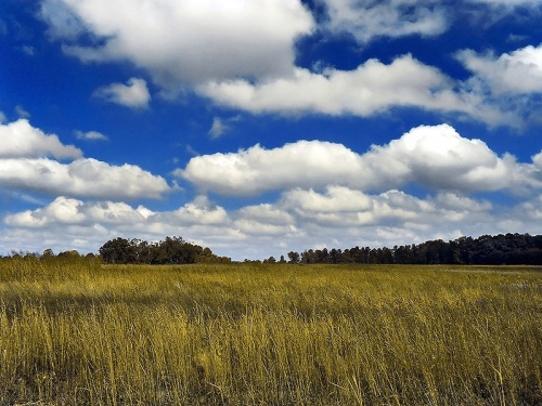
Anyway, a simple observation could be made for cumulus clouds by looking at such a sky :
There is almost no detail ! Cumulus clouds are mainly white at the top and gray at the bottom. Of course, light gets scattered and the clouds gets a bluish tint from the sky light. Also, photons bounce off from the ground and light the bottom of the cloud but, mainly, they are white and gray.
Basically, that means that we only need to know :
- The density of the cloud at a given position in space
- The accumulated density (or optical depth) the Sun light traversed to reach that position
Noise Precomputation
As I said earlier, I generally use a 16x16x16 noise texture that I combine at different frequencies (octaves) to obtain the turbulence noise pattern for my cloud density :
<math>\rho(x) = \sum_{i=0}^N \frac{Noise(2^i x)}{2^i}</math>
For my low resolution, low frequency clouds, I decided to use only 4 octaves. And to avoid tapping 4 noise values for every ray-marching step, I combined these 4 octaves of 16x16x16 noise into a single (4*16)x(4*16)x(4*16) = 128x128x128 texture. This way, I had a tiling noise texture that could give me the cloud density in a single tap.
As for the accumulated density, instead of creating a 128x128x128 R16F noise texture, I created a 128x128x128 RGBA16F texture. I had 3 more slots that I could read with the same texture tap. But what to put in those 3 slots ?
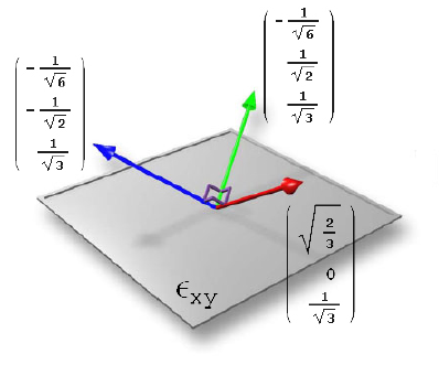
The answer : Radiosity Normal Maps. I mean, this is not really radiosity I was after, here. I simply recalled the idea of precomputing lighting for 3 main directions :
So that's what I did : I pre-computed for each noise cell, an average of the optical depth in 3 main directions. That would fail if the Sun ever went below the horizon but heck ! The yellow fellow is mainly above the clouds, and I could always hack the computation if it looked really bad at sunset... Which it didn't, so I didn't care about that.
That took about 2 hours of precomputation, that I later saved to disk and reloaded. I also tried to encode 3 SH coefficients (discarding ambient) but that would yield pretty much the same results except that it computed for 24h and never exited so I abandoned that idea.
Pre-computing noise data for hours is not something I like to do as it results in a large file on disk (24Mb uncompressed) and also makes the noise really static : no change is possible here ! I have to stick to the noise I precomputed. But that's a start.
In fact, only one change is possible and that's the one I was after : change in cloud coverage.
What does that mean ? For us, it simply comes to subtract a fixed value to the density : <math>\rho(x) = saturate( Noise(x) - Value )</math>.
But what does subtracting a constant value means for the 3 values of accumulated density ?
Well, the pre-computation of optical depth is simply :
<math>\tau(x,\vec\omega) = \int_0^D Noise(x + t \vec\omega) \, dt</math>

where :
<math>\vec\omega</math> is one the 3 main directions of precomputation
<math>D</math> is the distance to the exit point (i.e. top of the cloud layer) in that direction
If, instead, we integrate the noise density with the fixed offset, we get :
<math>\tau(x,\vec\omega,Value) = \int_0^D saturate( Noise(x + t \vec\omega) - Value ) \, dt</math>
I decided to ignore the nested saturate() part and write :
<math>\tau(x,\vec\omega,Value) \approx saturate( \int_0^D Noise(x + t \vec\omega) - Value \, dt ) = saturate( \int_0^D Noise(x + t \vec\omega) \, dt - Value * D )</math>
That's obviously wrong, but in practice that works pretty well. There is an obvious undershoot in the offseted accumulated density, that's why I tweaked the <math>- Value * D</math> part and used an empirical factor <math>D^\prime = \kappa \, D</math> instead.
Anyway, doing this allows us to retrieve an approximation of the optical depth with the noise offset, always with only a single texture tap.
What to trace ?
So, what is the scene we are going to render ? I created a test terrain that renders first in the ZBuffer so we can read back the depth of each pixel.
I decided to create a single layer of clouds sandwiched between 2 planes (I first tried with 2 spheres but I would have to ray-march along a curved line instead of a straight line so I abandoned the idea).
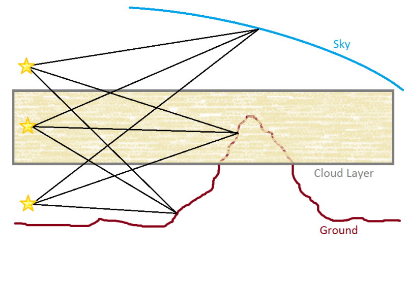
Here is a summary of the various configurations you will face when tracing a scene with a sky and a cloud layer :
The yellow stars represent 3 camera configurations : below, inside and above the clouds.
There is no real distinction between ground and sky here. If the depth at a pixel == ZFar then I considered it to be the upper atmosphere that I fixed at about 100km above see level. We can then simplify the problem if we label sky and ground as "obstacle".
We then end up with 5 categories of ray paths :
- Air <math>\to</math> Obstacle
- Air <math>\to</math> Cloud <math>\to</math> Obstacle
- Air <math>\to</math> Cloud <math>\to</math> Air <math>\to</math> Obstacle
- Cloud <math>\to</math> Obstacle
- Cloud <math>\to</math> Air <math>\to</math> Obstacle
It's pretty simple to compute these paths and the length for each of them. It's all a matter of ordering [0,CloudIn] [CloudIn,CloudOut] and [CloudOut,Infinity] intervals, where the "Obstacle" distance can interrupt these intervals early.
So all is left is tracing 3 zones : air above the clouds, the clouds themselves and air below the clouds.
Above Clouds
For air above clouds, I used pretty much the same code as Sean O'Neil, originally inspired by the article by Nishita et al. quoted earlier. I used about 8 ray-marching steps.
This code computes extinction and in-scattering for 2 atmospheric components : air molecules and aerosols (e.g. dust or fog microscopic water droplets).
The phase function used for the scattering of light by air molecules is the Rayleigh phase function : <math>p(\theta) = \frac{3}{4}(1+cos^2(\theta))</math>.
The phase function used for the scattering of light by aerosols is a simplification made by Christophe Shlick of the Henyey-Greenstein phase function : <math>p(\theta) = \frac{1-k^2}{(1+k cos(\theta))^2}</math>.
The density of these 2 components is a function of altitude and is given by :
<math>\rho(h) = e^{\frac{-h}{H0}}</math>

where :
h is the height in kilometers from sea level
H0 is a constant (different for air and aerosols)
Of course, this is only an approximation since this density increases when the sun goes down : gases are cooling down and become denser and heavier, accumulating at low altitudes. This is the reason why the sky and Sun are very red at dawn and sunset. But we can create the increase in density manually so a generic "daylight" model is quite okay.
I won't detail the technique here as many articles have already been written about sky models.
Clouds
When tracing the clouds, the routine is pretty much the same as the air described above except that, on top of air and aerosols, we also account for the cloud density.
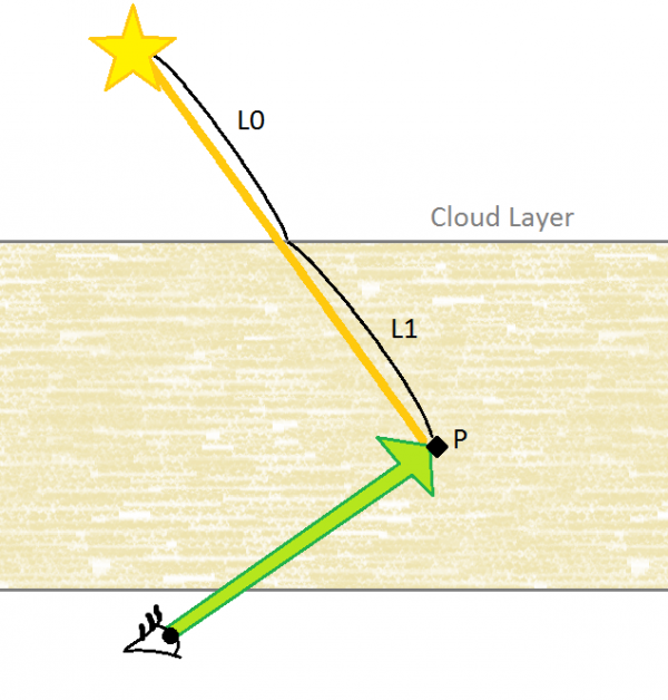
Ray-marching inside the cloud, we arrive at position P.
The algorithm then goes like this :
- We sample the noise density at P and also retrieve the accumulated densities in our 3 main directions, all from a single tap in our 128x128x128 RGBA16F texture.
- We compute the approximate accumulated density based on a weighted sum of the 3 main directions and the actual Sun direction
- The Sun light arriving at P is then :
- the original Sun light attenuated from the top of the atmosphere by air molecules and aerosols on a path of length L0 + L1, which I eagerly neglected.
- the original Sun light attenuated by traversing the cloud on a path of length L1
- We combine that attenuated Sun light with a phase function to obtain the single-scattered Sun light out going in the view direction (I'm using a combination of 3 Henyey-Greenstein phase functions here : strong forward, strong backward and medium "side")
To sum up :
<math>Li(P,\vec\omega) = \mathbf{p^\prime}(\widehat{\vec\omega \vec\omega_{sun}}) e^{-\tau(P,\vec\omega_{sun})} L_{sun}(\vec\omega_{sun})</math>

where :
<math>\tau(x,\vec\omega_{sun}) = \boldsymbol{\sigma} \boldsymbol{\rho}(x)</math>
<math>\boldsymbol{\sigma}</math> is the global cloud extinction factor
<math>\boldsymbol{\rho}(x)</math> is the accumulated density at <math>x</math> we talked about earlier
<math>\mathbf{p^\prime}(\theta)</math> is the combination of 3 phase functions
<math>\vec\omega_{sun}</math> is the direction toward the Sun
Don't forget that the total extinction for each ray marching step is the combination of extinction by air molecules, aerosols and cloud :
<math>Extinction = e^{-\tau_{air}} e^{-\tau_{aerosols}} e^{-\tau_{cloud}}</math>
And the same goes for in-scattering : in-scattered radiance is the sum of radiance from air molecules, aerosols and cloud particles.
<math>InScattering = \sigma_s \Delta_x \big[ L_i{air}(x,\vec\omega) p_{air}(\theta) + L_i{aerosols}(x,\vec\omega) p_{aerosols}(\theta) + L_i{cloud}(x,\vec\omega) p_{cloud}(\theta) \big]</math>
For accurate rendering I used 96 ray-marching steps for the clouds.
Below Clouds
Tracing below the clouds is exactly the same as tracing above them, except we sample the bottom of the clouds at each step to determine what energy is left after traversing the clouds. This is what creates the god rays : a difference in energy viewed through a curtain of dust and air.
God rays are only present if air is "polluted" (by dust or high air densities) and couldn't be seen otherwise. The same principle as a laser beam that can only be seen when bouncing off dust in the air.
So, that's pretty much the same as tracing air above the clouds except instead of using <math>L_{sun}(\vec\omega_{sun})</math> as the incoming Sun light, we use :
<math>L_{sun}^\prime(\vec\omega_{sun}) = L_{sun}(\vec\omega_{sun}) e^{-\tau_{cloud}(x^\prime,\vec\omega_{sun})}</math>

where :
<math>\tau_{cloud}(x^\prime,\vec\omega_{sun}) = \boldsymbol{\sigma} \boldsymbol{\rho}(x^\prime)</math>
<math>\boldsymbol{\rho}(x^\prime)</math> is the accumulated density, tapped from the cloud 3D texture at <math>x^\prime</math>
<math>x^\prime</math> is the projection of <math>x</math> (i.e. the current ray-marching position) onto the bottom of the cloud layer, as seen in the image below
Since we need to have a decent resolutions for god rays, I used 32 ray-marching steps when tracing below the clouds.
On a side note here, have you ever wondered why god rays seemed to emanate radially from the Sun whereas everyone tells you the Sun is so far away that it can be considered a directional light source ? They should be parallel, shouldn't they ? Well... It's really a matter of perspective :
Combining with an Existing Scene
As we have seen, the rendering takes place in a downscaled buffer. Recombining that buffer with the background scene is not as trivial as it seems.
My output for the cloud shader is written to 2 render targets (MRT) in RGBA16F format.
- The first RT contains XYZ = Extinction, W=Depth of the pixel
- The second RT contains XYZ = In-Scattering, W=Unused
I then use these 2 render targets as an input for the next stage : a fullscreen post-process combination with the original scene, also passed as an input.
The shader code (Shader Model 4.0) is :
float2 BufferInvSize; // X=1/OriginalBufferWidth Y=1/OriginalBufferHeight
float3 VolumeBufferInvSize; // X=1/DownsampledBufferWidth Y=1/DownsampledBufferHeight Z=0

float4  PS( float2 _ScreenPosition : SV_POSITION ) : SV_TARGET0
{
	float2	UV = _ScreenPosition.xy * BufferInvSize; // Normalize to [0,1]
	float4	SourceColor = SourceBuffer.SampleLevel( LinearClamp, UV, 0 ); // Read original scene's color
	float	Z = ReadDepth( UV );  // Read original scene's depth from the ZBuffer

	// =============================================
	// Perform an average of extinction & in-scattering values based on differences in Z : samples that are closest to actual depth will be used
	const float	Z_THRESHOLD = 10.0;

	// An array of 8 neighbor sample offsets
	float2	dUVs[] =
	{
		-VolumeBufferInvSize.xz,
		+VolumeBufferInvSize.xz,
		-VolumeBufferInvSize.zy,
		+VolumeBufferInvSize.zy,

		-VolumeBufferInvSize.xy,
		+VolumeBufferInvSize.xy,
		float2( VolumeBufferInvSize.x, -VolumeBufferInvSize.y ),
		float2( -VolumeBufferInvSize.x, VolumeBufferInvSize.y ),
	};

	float3	InScattering = 0.0;
	float4	ExtinctionZ = 0.0;
	float	SumWeights = 0.0;
	for ( int SampleIndex=0; SampleIndex < 8; SampleIndex++ )
	{
		float4	ExtinctionZSample = VolumeTextureExtinction.SampleLevel( LinearClamp, UV + dUVs[SampleIndex], 0 );
		if ( abs( ExtinctionZSample.w - Z ) > Z_THRESHOLD )
			continue; // That sample is not good enough : its depth is too far from the one of the pixel we computed

		float3	InScatteringSample = VolumeTextureInScattering.SampleLevel( LinearClamp, UV + dUVs[SampleIndex], 0 ).xyz;

		InScattering += InScatteringSample;
		ExtinctionZ += ExtinctionZSample;
		SumWeights++;
	}

	// Sample center
	float3	CenterInScattering = VolumeTextureInScattering.SampleLevel( LinearClamp, UV, 0 ).xyz;
	float4	CenterExtinctionZ = VolumeTextureExtinction.SampleLevel( LinearClamp, UV, 0 );
	if ( SumWeights == 0.0 || abs( CenterExtinctionZ.w - Z ) < Z_THRESHOLD )
	{
		InScattering += CenterInScattering;
		ExtinctionZ += CenterExtinctionZ;
		SumWeights++;
	}

	// We finally got our averaged extinction & in-scattering
	InScattering /= SumWeights;
	ExtinctionZ /= SumWeights;

	// =============================================
	// Compute Sun intensity
	float3	CameraView = normalize( float3( AspectRatio * TanHalfFOV * (2.0 * _ScreenPosition.x * BufferInvSize.x - 1.0), TanHalfFov * (1.0 - 2.0 * _ScreenPosition.y * BufferInvSize.y), 1.0 ) );
	float3	View = mul( float4( CameraView, 0.0 ), Camera2World ).xyz; // View vector in WORLD space

	float	CosAngle = 0.998;	            // Cos( SunCoverAngle )
	float	DotSun = dot( View, SunDirection ); // Phase with the Sun

	float	Infinity = FarClip - 5.0; // Arbitrary "infinite" distance
	float3	SunExtinction =
		ExtinctionZ.xyz *			// Color the Sun with extinction through atmosphere
		step( Infinity, ExtinctionZ.w ) *	// Don't display the Sun if it's behind the ZBuffer
		smoothstep( CosAngle, 1.0, DotSun );	// Make it smooth and not a sharp disk (although it should be)

	// =============================================
	// Combine Sun with original buffer
	return float4( SunExtinction * SunIntensity + InScattering + ExtinctionZ.xyz * SourceColor.xyz, SourceColor.w );
}
The Final Result
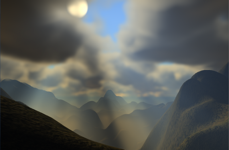
Here is a snapshot of the result :
(TODO: Find a better snapshot, that one is old)
And the video is available here http://www.youtube.com/watch?v=I1_f0z3Ht-k
Increasing realism, decreasing framerate : Deep Shadow Maps
Currently writing the code... Can't explain ! No time ! Rhaaa ! ![]()
Further research : multiple scattering precomputation
TODO
Further research : Lightning !
TODO
Further research : cumulo-nimbus clouds
TODO


