| (One intermediate revision by the same user not shown) | |||
| Line 1: | Line 1: | ||
| + | http://www.seas.ucla.edu/~vandenbe/133A/ | ||
| + | |||
| + | |||
== Matrix Decomposition Methods == | == Matrix Decomposition Methods == | ||
| Line 82: | Line 85: | ||
Computers usually ''solve square systems of linear equations'' using the LU decomposition, and it is also a key step when ''inverting a matrix'', or ''computing the determinant of a matrix''. | Computers usually ''solve square systems of linear equations'' using the LU decomposition, and it is also a key step when ''inverting a matrix'', or ''computing the determinant of a matrix''. | ||
| − | == Cholesky decomposition == | + | === Cholesky decomposition === |
[https://en.wikipedia.org/wiki/Cholesky_decomposition Cholesky Decomposition] => TODO | [https://en.wikipedia.org/wiki/Cholesky_decomposition Cholesky Decomposition] => TODO | ||
Latest revision as of 11:00, 5 August 2017
http://www.seas.ucla.edu/~vandenbe/133A/
Contents
[hide]Matrix Decomposition Methods
QR Decomposition
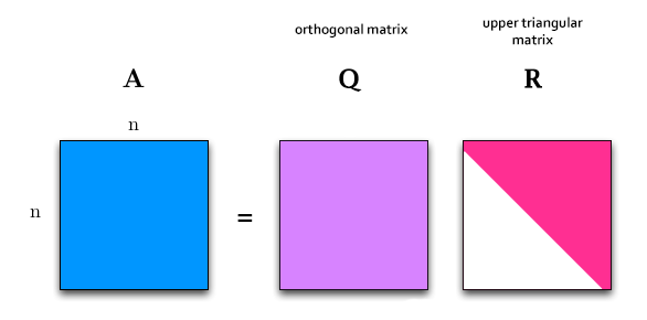
QR Decomposition, or QR Factorization is the process of decomposing a square matrix A this way: <math>\left [ \bold{A} \right ] = \left [ \bold{Q} \right ] \cdot \left [ \bold{R} \right ]</math>
Where:
- Q is an orthogonal matrix
- R is an upper triangular matrix
Applications
QR decomposition is often used to solve the linear least squares problem, and is the basis for a particular eigenvalue algorithm, the QR algorithm.
SVD Decomposition
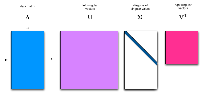
Singular Value Decomposition (SVD) is the process of decomposing a matrix A this way:
<math>\left [ \bold{A} \right ] = \left [ \bold{U} \right ] \cdot \left [ \bold{\Sigma} \right ] \cdot \left [ \bold{V} \right ]^T</math>
Where:
- A is an <math>m \times n</math> real or complex matrix
- U is an <math>m \times m</math> real or complex unitary orthonormal matrix
- <math>\bold{\Sigma}</math> is an <math>m \times n</math> rectangular diagonal matrix with non-negative real numbers on the diagonal
- V is an <math>n \times n</math> real or complex unitary orthonormal matrix.
NOTES:
- The diagonal entries <math>\sigma_i</math> of <math>\bold{\Sigma}</math> are known as the singular values of A and can be viewed as the semiaxes of an n-dimensional ellipsoid.
- The columns of U and the columns of V are called the left-singular vectors and right-singular vectors of A, respectively.
The singular value decomposition can be computed using the following observations:
- The left-singular vectors of A are a set of orthonormal eigenvectors of <math>\bold{A}\bold{A}^T</math>.
- The right-singular vectors of A are a set of orthonormal eigenvectors of <math>\bold{A}^T\bold{A}</math>.
- The non-zero singular values of A (found on the diagonal entries of Σ) are the square roots of the non-zero eigenvalues of both <math>\bold{A}^T\bold{A}</math> and <math>\bold{A}\bold{A}^T</math>.
Applications
Applications that employ the SVD include computing the pseudoinverse, least squares fitting of data, multivariable control, matrix approximation, and determining the rank, range and null space of a matrix.
LU Decomposition
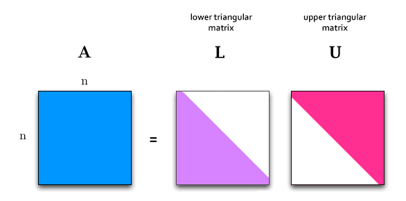
LU Decomposition, or LU Factorization can be viewed as the matrix form of Gaussian elimination. It is the process of decomposing a square matrix A this way: <math>\left [ \bold{A} \right ] = \left [ \bold{L} \right ] \cdot \left [ \bold{U} \right ]</math>
Where:
- L is a Lower triangular matrix
- U is an Upper triangular matrix
<math>
\begin{bmatrix}
          a_{11} & a_{12} & a_{13} \\
          a_{21} & a_{22} & a_{23} \\
          a_{31} & a_{32} & a_{33}
       \end{bmatrix} =
     \begin{bmatrix}
          l_{11} & 0 & 0 \\
          l_{21} & l_{22} & 0 \\
          l_{31} & l_{32} & l_{33}
       \end{bmatrix}
       \begin{bmatrix}
          u_{11} & u_{12} & u_{13} \\
          0 & u_{22} & u_{23} \\
          0 & 0 & u_{33}
       \end{bmatrix}.
</math>
Applications
Computers usually solve square systems of linear equations using the LU decomposition, and it is also a key step when inverting a matrix, or computing the determinant of a matrix.
Cholesky decomposition
Cholesky Decomposition => TODO
Applications
Useful for efficient numerical solutions and Monte Carlo simulations. When it is applicable, the Cholesky decomposition is roughly twice as efficient as the LU decomposition for solving systems of linear equations.


