| (9 intermediate revisions by the same user not shown) | |||
| Line 3: | Line 3: | ||
Maybe you already bumped into the problem of projecting a cubemap into spherical harmonics and found this page to help you out: http://www.rorydriscoll.com/2012/01/15/cubemap-texel-solid-angle/ ? | Maybe you already bumped into the problem of projecting a cubemap into spherical harmonics and found this page to help you out: http://www.rorydriscoll.com/2012/01/15/cubemap-texel-solid-angle/ ? | ||
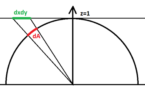
| − | [[File:PerspectiveProjection.png|500px|Perspective projection of an area element on plane z=1 onto the hemisphere]] | + | [[File:PerspectiveProjection.png|500px|Figure 1. : Perspective projection of an area element on plane z=1 onto the hemisphere]] |
But maybe you need the solution to another, similar problem that consists in finding the solid angle of a pixel lying in the z=0 plane and orthogonally projected onto the hemisphere, but couldn't find a page with that computation? | But maybe you need the solution to another, similar problem that consists in finding the solid angle of a pixel lying in the z=0 plane and orthogonally projected onto the hemisphere, but couldn't find a page with that computation? | ||
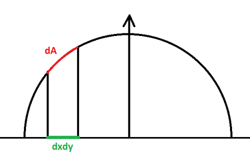
| − | [[File:OrthoProjection.png|500px|Orthographic projection of an area element on plane z=0 onto the hemisphere]] | + | [[File:OrthoProjection.png|500px|Figure 2. : Orthographic projection of an area element on plane z=0 onto the hemisphere]] |
| Line 18: | Line 18: | ||
==Cubemap Projection Configuration== | ==Cubemap Projection Configuration== | ||
| − | The configuration for a cube map is that pixels are lying on a plane z=1 such as <math>\mathbf{p'}=(x,y,1), -1<x<1, -1<y<1</math> and we project back onto the unit hemisphere by | + | The configuration for a cube map is that pixels are lying on a plane z=1 such as <math>\mathbf{p'}=(x,y,1), -1<x<1, -1<y<1</math> and we project back onto the unit hemisphere by normalizing the vector <math>\mathbf{p}=\frac{\mathbf{p'}}{|\mathbf{p'}|}=\frac{(x,y,1)}{\sqrt{1+x^2+y^2}}</math> as shown on figure 1 above. |
The idea is to compute the area of a small element of surface on the hemisphere as we make it vary on the plane, we do that by computing the partial derivatives of <math>\mathbf{p}</math> along x and y that give us the vectors <math>\frac{\partial \mathbf{p}}{\partial x}</math> and <math>\frac{\partial \mathbf{p}}{\partial y}</math>. | The idea is to compute the area of a small element of surface on the hemisphere as we make it vary on the plane, we do that by computing the partial derivatives of <math>\mathbf{p}</math> along x and y that give us the vectors <math>\frac{\partial \mathbf{p}}{\partial x}</math> and <math>\frac{\partial \mathbf{p}}{\partial y}</math>. | ||
| − | + | It is well-known to graphics programmers that computing the cross product of these vectors gives us the normal to the sphere at position <math>\mathbf{p}</math>, and the length of that normal is the tiny area element <math>dA</math> on the hemisphere. | |
Integrating this operation (cross product and norm computation) over an interval <math>[a,b]\in\mathbb{R}^2</math> yields: | Integrating this operation (cross product and norm computation) over an interval <math>[a,b]\in\mathbb{R}^2</math> yields: | ||
<math>A(x,y) = \int_0^y \int_0^x \left | \frac{\partial \mathbf{p}}{\partial x} \times \frac{\partial \mathbf{p}}{\partial y} \right | \, da \, db \\ | <math>A(x,y) = \int_0^y \int_0^x \left | \frac{\partial \mathbf{p}}{\partial x} \times \frac{\partial \mathbf{p}}{\partial y} \right | \, da \, db \\ | ||
| − | = \int_0^y \int_0^x (1+a^2+b^2)^{-\frac{3}{2}} \, da \, db \\ | + | = \int_0^y \int_0^x \left (1+a^2+b^2 \right )^{-\frac{3}{2}} \, da \, db \\ |
= \left | atan( \frac{xy}{\sqrt{1+x^2+y^2}} ) \right | \quad \quad \quad (1) | = \left | atan( \frac{xy}{\sqrt{1+x^2+y^2}} ) \right | \quad \quad \quad (1) | ||
</math> | </math> | ||
| − | It's easy to notice that <math>A(1,1) = \frac{\pi}{6}</math> which is the solid angle covered by a quarter of our cube map face, the solid angle of an | + | It's easy to notice that <math>A(1,1) = \frac{\pi}{6}</math> which is the solid angle covered by a quarter of our cube map face, the solid angle of an entire face would be <math>\frac{2\pi}{3}</math> and all 6 faces of the cube map are then covering a proper solid angle of <math>4\pi</math> and all is well! |
| Line 63: | Line 63: | ||
Except the primitive of this expression is a bit of nightmare after all, but this is our final result: | Except the primitive of this expression is a bit of nightmare after all, but this is our final result: | ||
{| class="wikitable" align="center" | {| class="wikitable" align="center" | ||
| − | | style="background: Periwinkle;" | <math>A(x,y) = \int_0^y \int_0^x \frac{1}{\sqrt{1-a^2-b^2}} da \, db = \tan ^{-1}\left(\frac{x}{\sqrt{-x^2-y^2+1}}\right)+x \tan ^{-1}\left(\frac{y}{\sqrt{-x^2-y^2+1}}\right)+\frac{1}{2} \left(\tan ^{-1}\left(\frac{-x-y^2+1}{y \sqrt{-x^2-y^2+1}}\right)-\tan ^{-1}\left(\frac{x-y^2+1}{y \sqrt{-x^2-y^2+1}}\right)\right) \quad \quad \quad (2)</math> | + | | style="background: Periwinkle;" | <math>A(x,y) = \int_0^y \int_0^x \frac{1}{\sqrt{1-a^2-b^2}} da \, db = y \tan ^{-1}\left(\frac{x}{\sqrt{-x^2-y^2+1}}\right) + x \tan ^{-1}\left(\frac{y}{\sqrt{-x^2-y^2+1}}\right)+\frac{1}{2} \left(\tan ^{-1}\left(\frac{-x-y^2+1}{y \sqrt{-x^2-y^2+1}}\right)-\tan ^{-1}\left(\frac{x-y^2+1}{y \sqrt{-x^2-y^2+1}}\right)\right) \quad \quad \quad (2)</math> |
|} | |} | ||
| Line 87: | Line 87: | ||
Say you have the normalized expression of a Normal Distribution Function D(x,y) defined in an image of the flattened hemisphere: | Say you have the normalized expression of a Normal Distribution Function D(x,y) defined in an image of the flattened hemisphere: | ||
| − | [[File: | + | [[File:Fabric_weave_NDF_normalized.png|300px]] |
| + | |||
And you want to compute the shadowing/masking term as given by [https://hal.inria.fr/hal-01168516v2/document Dupuy et al] eq. 3: | And you want to compute the shadowing/masking term as given by [https://hal.inria.fr/hal-01168516v2/document Dupuy et al] eq. 3: | ||
| Line 95: | Line 96: | ||
All you have to do is to write a convolution for each pixel of the image with a code similar to this: | All you have to do is to write a convolution for each pixel of the image with a code similar to this: | ||
| + | |||
| + | // Perform an integration with the NDF weighted by the cosine of the angle with that particular direction | ||
| + | float3 k = given; | ||
| + | float3 h; | ||
| + | float convolution = 0.0; | ||
| + | for ( uint Y=0; Y < Height; Y++ ) { | ||
| + | h.y = 2.0f * Y / Height - 1.0f; | ||
| + | for ( uint X=0; X < Width; X++ ) { | ||
| + | h.x = 2.0f * X / Width - 1.0f; | ||
| + | float sqSinTheta = h.x*h.x + h.y*h.y; | ||
| + | if ( sqSinTheta >= 1.0f ) | ||
| + | continue; | ||
| + | |||
| + | h.z = sqrt( 1.0f - sqSinTheta ); | ||
| + | |||
| + | float k_o_h = k.Dot( h ); // k.h | ||
| + | float D = NDF[X,Y].x; // D(h) | ||
| + | float dW = ComputeArea( X, Y ); // dW | ||
| + | |||
| + | convolution += k_o_h * D * dW; | ||
| + | } | ||
| + | } | ||
| + | float G = k.z / convolution; | ||
| − | This yields the G term as an image, | + | This yields the G term as an image that I'm showing here with a strong contrast applied, otherwise it's mostly white: |
| − | [[File: | + | [[File:Fabric_weave_G_contrasted.png|300px]] |
Latest revision as of 18:43, 7 June 2017
Hi!
Maybe you already bumped into the problem of projecting a cubemap into spherical harmonics and found this page to help you out: http://www.rorydriscoll.com/2012/01/15/cubemap-texel-solid-angle/ ?
But maybe you need the solution to another, similar problem that consists in finding the solid angle of a pixel lying in the z=0 plane and orthogonally projected onto the hemisphere, but couldn't find a page with that computation?
Well let me help you with that! ![]()
First of all, the document that was used initially to do the computations -- whether it be in AMD's cube map generator, Rory Driscoll's summary or this page -- is the very interesting thesis by Manne Öhrström.
Contents
Cubemap Projection Configuration
The configuration for a cube map is that pixels are lying on a plane z=1 such as <math>\mathbf{p'}=(x,y,1), -1<x<1, -1<y<1</math> and we project back onto the unit hemisphere by normalizing the vector <math>\mathbf{p}=\frac{\mathbf{p'}}{|\mathbf{p'}|}=\frac{(x,y,1)}{\sqrt{1+x^2+y^2}}</math> as shown on figure 1 above.
The idea is to compute the area of a small element of surface on the hemisphere as we make it vary on the plane, we do that by computing the partial derivatives of <math>\mathbf{p}</math> along x and y that give us the vectors <math>\frac{\partial \mathbf{p}}{\partial x}</math> and <math>\frac{\partial \mathbf{p}}{\partial y}</math>.
It is well-known to graphics programmers that computing the cross product of these vectors gives us the normal to the sphere at position <math>\mathbf{p}</math>, and the length of that normal is the tiny area element <math>dA</math> on the hemisphere.
Integrating this operation (cross product and norm computation) over an interval <math>[a,b]\in\mathbb{R}^2</math> yields:
<math>A(x,y) = \int_0^y \int_0^x \left | \frac{\partial \mathbf{p}}{\partial x} \times \frac{\partial \mathbf{p}}{\partial y} \right | \, da \, db \\ = \int_0^y \int_0^x \left (1+a^2+b^2 \right )^{-\frac{3}{2}} \, da \, db \\ = \left | atan( \frac{xy}{\sqrt{1+x^2+y^2}} ) \right | \quad \quad \quad (1) </math>
It's easy to notice that <math>A(1,1) = \frac{\pi}{6}</math> which is the solid angle covered by a quarter of our cube map face, the solid angle of an entire face would be <math>\frac{2\pi}{3}</math> and all 6 faces of the cube map are then covering a proper solid angle of <math>4\pi</math> and all is well!
Now, for our little problem...
Our Projection Configuration
Our configuration is a little bit different as our points <math>\mathbf{p'}(x,y) = (x,y,0)</math> and we project onto the hemisphere to obtain <math>\mathbf{p}(x,y) = (x,y,\sqrt{1-x^2-y^2})</math>.
The partial derivatives along x and y give:
<math>\frac{\partial \mathbf{p}}{\partial x} = \begin{pmatrix} 1 \\ 0 \\ -\frac{x}{\sqrt{1-x^2-y^2}} \end{pmatrix}</math>
<math>\frac{\partial \mathbf{p}}{\partial y} = \begin{pmatrix} 0 \\ 1 \\ -\frac{y}{\sqrt{1-x^2-y^2}} \end{pmatrix}</math>
The cross product of these 2 vectors gives:
<math>\frac{\partial \mathbf{p}}{\partial x} \times \frac{\partial \mathbf{p}}{\partial y} = \frac{1}{\sqrt{1-x^2-y^2}} \begin{pmatrix} x \\ y \\ \sqrt{1-x^2-y^2} \end{pmatrix}</math>
And the norm is:
<math>\left | \frac{\partial \mathbf{p}}{\partial x} \times \frac{\partial \mathbf{p}}{\partial y} \right | = \frac{1}{\sqrt{1-x^2-y^2}}</math>
Which looks kinda nice! Integrating where it is definite (i.e. with x and y in the unit circle) <math>\int_0^1\int_0^1 \frac{1}{\sqrt{1-x^2-y^2}} dx \, dy = \frac{\pi}{2}</math> which is a quarter of the entire hemisphere's solid angle <math>2\pi</math>, so we're good!
Except the primitive of this expression is a bit of nightmare after all, but this is our final result:
| <math>A(x,y) = \int_0^y \int_0^x \frac{1}{\sqrt{1-a^2-b^2}} da \, db = y \tan ^{-1}\left(\frac{x}{\sqrt{-x^2-y^2+1}}\right) + x \tan ^{-1}\left(\frac{y}{\sqrt{-x^2-y^2+1}}\right)+\frac{1}{2} \left(\tan ^{-1}\left(\frac{-x-y^2+1}{y \sqrt{-x^2-y^2+1}}\right)-\tan ^{-1}\left(\frac{x-y^2+1}{y \sqrt{-x^2-y^2+1}}\right)\right) \quad \quad \quad (2)</math> |
I tried to further out the simplification of the last 2 atan terms since a difference of atan gives a single atan but it turns out it shows some precision issues.
How to use this?
As explained by Driscoll, we compute the area of a single pixel by doing the exact same operation as with Summed Area Tables, that is we compute 4 values for the area of 4 sections like shown here:
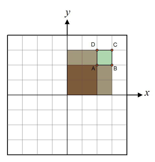
Then we get: <math>dA(x,y) = C + A - D - B</math>
NOTE:
- Obviously, you have to be very careful not to use eq. (2) outside of its region of definition <math>x^2+y^2 < 1</math>
- Trying to compute the hemisphere's area using eq. (2) turns out to be converging super slowly: even with a quarter disc split into 10000x10000 pixels, I can only reach 1.5535995614989679...
Example
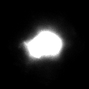
Say you have the normalized expression of a Normal Distribution Function D(x,y) defined in an image of the flattened hemisphere:
And you want to compute the shadowing/masking term as given by Dupuy et al eq. 3:
<math>G(\mathbf{k}) = \frac{cos \theta_k}{\int_{\Omega_+}{\mathbf{k}\mathbf{h} \, D(\mathbf{h}}) \, d\omega_h}</math>
All you have to do is to write a convolution for each pixel of the image with a code similar to this:
// Perform an integration with the NDF weighted by the cosine of the angle with that particular direction
float3 k = given;
float3 h;
float  convolution = 0.0;
for ( uint Y=0; Y < Height; Y++ ) {
  h.y = 2.0f * Y / Height - 1.0f;
  for ( uint X=0; X < Width; X++ ) {
    h.x = 2.0f * X / Width - 1.0f;
    float  sqSinTheta = h.x*h.x + h.y*h.y;
    if ( sqSinTheta >= 1.0f )
      continue;

    h.z = sqrt( 1.0f - sqSinTheta );

    float  k_o_h = k.Dot( h );         // k.h
    float  D = NDF[X,Y].x;             // D(h)
    float  dW = ComputeArea( X, Y );   // dW

    convolution += k_o_h * D * dW;
  }
}
float	G = k.z / convolution;
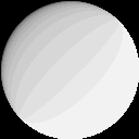
This yields the G term as an image that I'm showing here with a strong contrast applied, otherwise it's mostly white:
